Graph Theory
Contents
Introduction
In real life, connections can be made in numerous situations such as subway routes connecting one city to another. Graphs can be used to model these connections.
Terminology
A graph is a collection of vertices (or nodes) and edges. An edge is a line used to connect two vertices to each other.
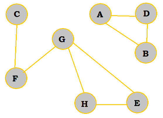
A graph should not be defined by its visual representation but rather by its set of vertices of edges. This is because there are numerous ways to visually display the same graph; see the example below.
| Version 1 | Version 2 |
|---|---|
 |
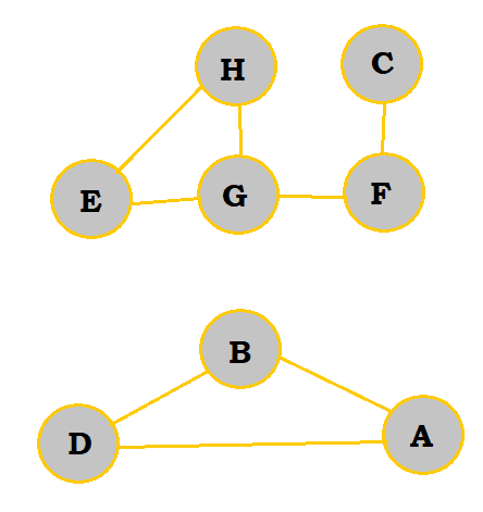 |
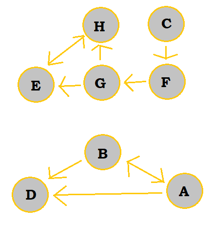
So, rather than defining the graph above by giving its visual, it would be better to state that its set of vertices is {A, B, C, D, E, F, G}, and its set of edges is {AB, AD, BD, CF, FG, GH, GE, HE}.
A path in a graph is a list of successive vertices connected by edges in a graph. The vertices should be listed in the order that they are traveled in to make the path. For example, FGHE and FGE are both valid paths for going from vertex F to vertex E in the above graph.
A simple path is a path with no vertex repeated. FGHE is an example of a simple path. The opposite of a simple path would be a cycle, a path where the first and last vertex are the same (essentially a path that points back to itself). ABDA is an example of a cycle. The same cycle can be depicted in multiple ways; for example, BDAB is the same as ABDA except that it starts on a different vertex.
Note: It is very important to be able to recognize whether two cycles are the same or not as identifying the number of distinct cycles in a graph is a commonly asked question.
Classifying Graphs
Graphs can be drawn a number of ways depending on its set of vertices and set of edges. To better describe graphs, we look for particular characteristics to classify them. Please read the sections below for more detail.
Graph Density
In many cases, there may not be an edge to connect a vertex to every other vertex directly; instead, paths must be taken to get from one vertex to another.
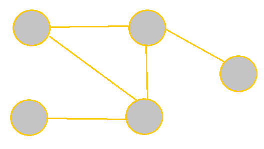
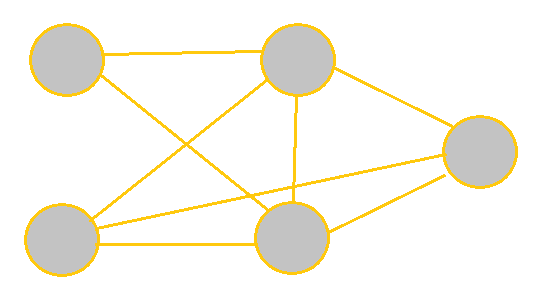
Sparse graphs are graphs that have relatively few edges present, whereas dense graphs have most edges present. Complete graphs have all edges present. 'All edges' means that there is an edge connecting every pair of vertices.
| Sparse | Dense | Complete |
|---|---|---|
 |
 |
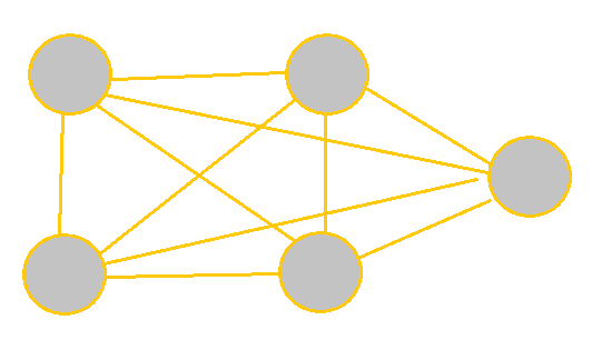 |
Directed Paths
Directed graphs are those that have a direction associated with each edge. So, an edge from X to Y would not be the same as an edge from Y to X. For edges with arrows on both ends, this would mean that the edge goes both ways. A directed graph with no cycles can be referred to as a dag, which stands for "directed acyclic graph".
Undirected graphs are graphs where all edges can go both ways. So, they are essentially graphs where the edges all have dual arrows on both ends.
Unless arrows are present on the edges, or the problem indicates it specifically, assume any graph given to you is an undirected graph.
Weighted Graphs
Weighted graphs are those where each edge has a numerical weight/cost associated with it. These weights are usually positive integers. They can be either directed or undirected.
In applications, these can represent the length of a route between two cities or perhaps the cost of a plane ticket between two countries.
Trees
A tree is a graph that contains no cycles, meaning that there is only one path between any two nodes. A tree with N vertices has exactly N-1 edges, unlike regular graphs, which can vary in how many edges they have.
A spanning tree of a graph is a tree that contains all of the vertices of a graph. A minimal spanning tree is the spanning tree that has the minimum cost, which is calculated by the sum of all the edges in the tree. Naturally, the minimal spanning tree can only be found in a weighted graph.
A group of disconnected trees is called a forest.
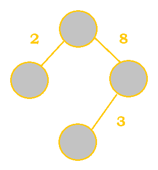
| Weighted Graph |
|---|
 |
| Spanning Tree |
|---|
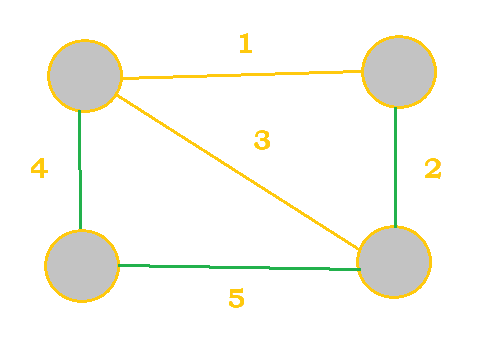 Cost $= 4 + 5 + 2 = 11$ |
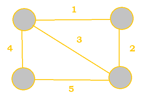
| Minimum Spanning Tree |
|---|
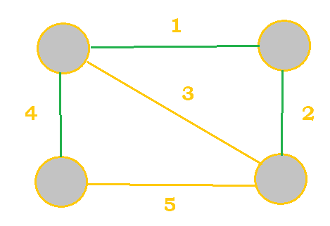 Cost $= 4 + 1 + 2 = 7$ |
Adjacency Matrices
Matrices are very useful when it comes to depicting a graph. They are a more numerical way to represent a graph. They are specifically useful for knowing how many paths of a certain length exist between any two vertices.
Writing the Graph as a Matrix
Let's create an example. Let's say that we had this graph:
To start off, our template matrix would look like so:
| A | B | C | |
|---|---|---|---|
| A | |||
| B | |||
| C |
Note that the letters are simply written as a reference; they are not part of the actual matrix. The letters written vertically represent starting locations. The letters written horizontally represent destinations.
Then, we fill out our matrix with 0s and 1s, with 1 signifying that an edge connects the vertices in its column and row. So, for example, in the top right empty box, this would
be filled out with a 1 because there is indeed an edge that goes from A to C. Pay careful attention to which box there is a $1$ in for directed graphs as sometimes there is an edge connecting B to C but not C to B.
So, the rest of the matrix will be filled out as follows:
| A | B | C | |
|---|---|---|---|
| A | $1$ |
$0$ |
$1$ |
| B | $0$ |
$1$ |
$1$ |
| C | $1$ |
$0$ |
$0$ |
Powers of a Matrix
Before moving to adjacency matrices, it is crucial that you know how to find the power of a matrix, which is just multiplying a matrix by itself a certain number of times. If you already know how to do so, please feel free to skip to the next section.
Let's say that we have two matrices, A and B. A is a 2 x 3 matrix, whereas 3 x 2 matrix. If we were to multiply these
two matrices together, the resultant matrix's dimension would be 2 x 2. This is because dimensions follow this
concept: $(m \: x \: n) \bullet (n \: x \: k) = (m \: x \: k)$. This rule must be followed; the number of columns in the first matrix
must match the number of rows in the second matrix for matrix multiplication to work properly.
Now, for actually multiplying matrices, you will need to use the dot product. Let's specify matrices A and B a bit further:
| A | ||
|---|---|---|
| 1 | 2 | 3 |
| 4 | 5 | 6 |
| B | |
|---|---|
| 6 | 3 |
| 5 | 2 |
| 4 | 1 |
To start off, we will work with the first row of the first matrix and the first column of the second matrix. 1 is multiplied by 6, 2 is multiplied by 5, and 3 is multiplied by 4; notice how we worked from left to right for the row and top to bottom for the column.
Then, the sum of these products are added together; this sum then becomes the first element of the first row of the resultant matrix. You would then move to multiplying the first row of the first matrix with the second column of the second matrix in the same manner; this would get you the second element of the first row of the resultant matrix.
This can be quite hard to understand at first, so please use this visualization to help out:
$A \bullet B$ |
|
|---|---|
$(1 \bullet 6) + (2 \bullet 5) + (3 \bullet 4)$ |
$(1 \bullet 3) + (2 \bullet 2) + (3 \bullet 1)$ |
$(4 \bullet 6) + (5 \bullet 5) + (6 \bullet 4)$ |
$(4 \bullet 3) + (5 \bullet 2) + (6 \bullet 1)$ |
This would then ultimately simplify to:
$A \bullet B$ |
|
|---|---|
| 28 | 10 |
| 73 | 28 |
Setting Up an Adjacency Matrix
Now, with matrix multiplication, you can now set up adjacency matrices! This is how it works. Let's say we have the
matrix M and would like to know how many paths of length 2 exist between two specific vertices. So, we would calculate
$M^2$, or $M \bullet M$. Our new numbers would get us our answer.
Let's use the following graph once more:
As we calculated before, the matrix would be:
$M$ |
A | B | C |
|---|---|---|---|
| A | 1 | 0 | 1 |
| B | 0 | 1 | 1 |
| C | 1 | 0 | 0 |
Then, we would have to multiply this by itself once to get $M^2$.
$M^2$ |
A | B | C |
|---|---|---|---|
| A | $(1 \bullet 1) + (0 \bullet 0) + (1 \bullet 1)$ |
$(1 \bullet 0) + (0 \bullet 1) + (1 \bullet 0)$ |
$(1 \bullet 1) + (0 \bullet 1) + (1 \bullet 0)$ |
| B | $(0 \bullet 1) + (1 \bullet 0) + (1 \bullet 1)$ |
$(0 \bullet 0) + (1 \bullet 1) + (1 \bullet 0)$ |
$(0 \bullet 1) + (1 \bullet 1) + (1 \bullet 0)$ |
| C | $(1 \bullet 1) + (0 \bullet 0) + (0 \bullet 1)$ |
$(1 \bullet 0) + (0 \bullet 1) + (0 \bullet 0)$ |
$(1 \bullet 1) + (0 \bullet 1) + (0 \bullet 0)$ |
So, the matrix squared would be:
$M^2$ |
A | B | C |
|---|---|---|---|
| A | 2 | 0 | 1 |
| B | 1 | 1 | 1 |
| C | 1 | 0 | 1 |
So, there are 2 paths of length 2 that go from A to itself. There are no paths of length 2 that go from A to B. Similar
conclusions can be made for the rest of the numbers. if you were to find $M^3$ or $M^4$ instead, you would find the number of paths of lengths 3 and 4, respectively, that connect two given vertices. This idea is very useful when ACSL asks to find all cycles or paths of a certain lengths, since manually counting the number of paths is a tedious and error-prone process (See example question 3).
Sample Problems
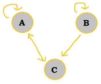
1. How many different cycles are contained in the directed graph visualized below:
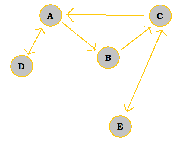
One cycle is ADA, or DAD. Another is ABCA, which is also BCAB or CABC. The last cycle is ECE, or CEC. So, in total, there are 3 different cycles in the graph.
2. Using the adjacency matrix below, draw the directed graph.
$M$ |
A | B | C | D | E |
|---|---|---|---|---|---|
| A | 1 | 0 | 1 | 1 | 0 |
| B | 0 | 1 | 0 | 1 | 1 |
| C | 0 | 0 | 0 | 1 | 0 |
| D | 0 | 1 | 1 | 0 | 1 |
| E | 1 | 0 | 1 | 1 | 1 |
The drawn graph below is only one way to depict this matrix. You can place the nodes anywhere you'd like.
| Step | Graph |
|---|---|
| Draw in A's edges | 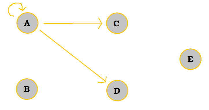 |
| Add B's edges | 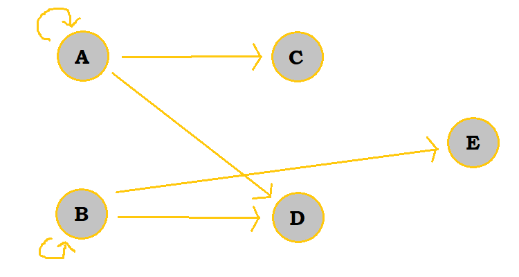 |
| Add C's edges | 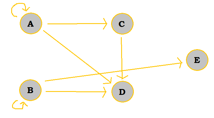 |
| Add D's edges | 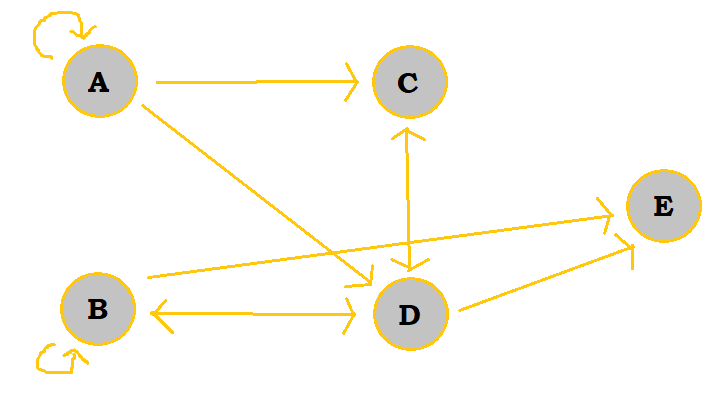 |
| Add E's edges | 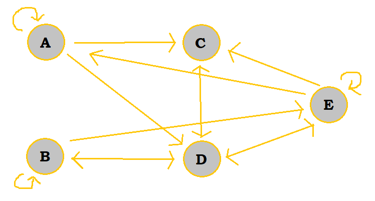 |
3. In the following directed graph, find the total number of different paths from vertex B to vertex D of length 3.
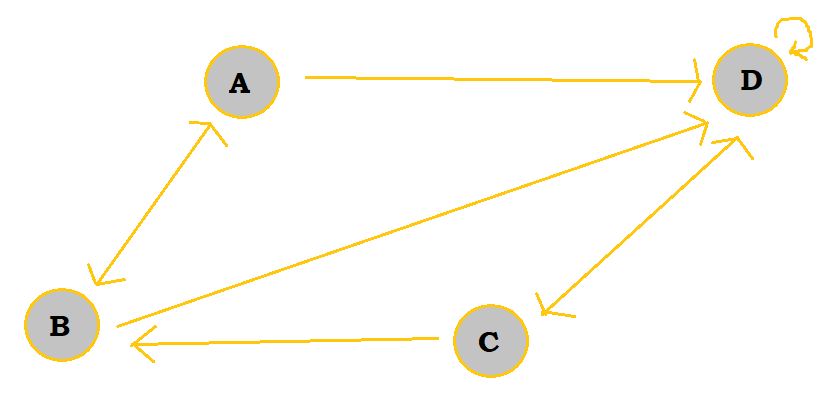
First, let's start with writing the graph as a regular matrix:
$M$ |
A | B | C | D |
|---|---|---|---|---|
| A | 0 | 1 | 0 | 1 |
| B | 1 | 0 | 0 | 1 |
| C | 0 | 1 | 0 | 1 |
| D | 0 | 0 | 1 | 1 |
Then, we can multiply this by itself to first get $M^2$.
$M^2$ |
A | B | C | D |
|---|---|---|---|---|
| A | 1 | 0 | 1 | 2 |
| B | 0 | 1 | 1 | 2 |
| C | 1 | 0 | 1 | 2 |
| D | 0 | 1 | 1 | 2 |
Finally, we can multiply $M^2$ by $M$ to get $M^3$.
$M^3$ |
A | B | C | D |
|---|---|---|---|---|
| A | 0 | 2 | 2 | 4 |
| B | 1 | 1 | 2 | 4 |
| C | 0 | 2 | 2 | 4 |
| D | 1 | 1 | 2 | 4 |
So, there are 4 total paths of length 3 from B to D. If we were to manually solve this with a matrix, we would come to the same conclusion. The paths are: BADD, BDDD, BABD, and BDCD.
Author: Kelly Hong