Data Structures

Contents

• Introduction
• Stacks and Queues
  • Stacks
  • Queues
• Trees
  • Terminology
  • Binary Search Trees
  • Inserting Nodes (Binary Search)
  • Deleting Nodes (Binary Search)
  • Searching for Nodes
  • Classifying Trees Further
  • Balanced Trees
  • Full vs Complete Trees
• Path Lengths
• Priority Queues
  • Inserting Nodes (Priority Queues)
  • Deleting Nodes (Priority Queues)
• Sample Problems

Introduction

Data structures are an integral part of efficient algorithms. When you have a large amount of data to work with, data structures help you keep organized and manage everything properly; knowing the right data structure to use will ensure you don't waste resources when running your program.

ACSL specifically focuses on stacks, queues, binary search trees, and priority queues. The general idea behind each is covered but not the actual details regarding how to implement them in programs.

For programming, there is a much more useful section on data structures (to come).

Stacks and Queues

Stacks

Stacks are generally used to save information to be processed later on. This applies to recursion (when a function calls on itself); the inner function call comes after the actual function call but is processed first.

Stacks work in a "last in, first out" (LIFO) order. They support two operations, PUSH and POP. PUSH takes in a key, which is essentially a parameter, to insert at the top of the stack. So, PUSH("A") would add the key "A" to the top of the stack. POP is a bit different, as it is written as X = POP(). What this does is that it removes the top element in the stack and stores it in variable X. So, if there was a stack with its top element being "E", then writing H = POP() would store "E" in H.

In the case that the POP operation is called on an empty stack, then the variable is given the special value NIL (Not In List), which means "nonexistent".

Queues

Queues, on the other hand, are often used to handle requests. It's similar to waiting in line (or a queue); the first people in line are processed first. Hence, queues follow a "first in, first out" (FIFO) order.

The PUSH operation works the same as it would with stacks (the element is added to the top of the data structure). However, with POP, instead of removing the top (most recently added) element, queues have their bottom element removed.

A tip to handle both queue and stack related problems is to keep a list of all the elements, with the pushed elements being added to the top of the list. In a queue, cross off the bottom element, and in a stack cross off the top element.

Trees

Terminology

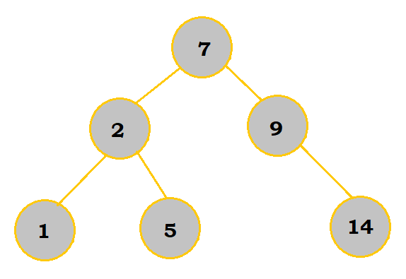
Trees consist of elements called nodes that are connected by edges. The root is the top node in the tree. Parent nodes are nodes that have other nodes, children nodes, stemming from them. Leaves are the nodes that do not have any other children nodes stemming from them. Nodes that have the same immediate parent are siblings.

So, in the following table below, 7 is the root. 7, 2, and 9 are all parent nodes, 2, 9, 1, 5, and 14 are all children nodes (notice that parent nodes can also be children of other nodes), 1, 5, and 14 are leaves, and 1 and 5 are siblings.

Binary Search Trees

Binary search trees are one way to store items in a particular order. They can efficiently insert, delete, and look for items within the tree.

Each node can have a total of two children. The left child must be less than or equal in value, whereas the right child must be greater in value. With numbers, this is easy enough; as for alphabet letters, they are considered to be "less than" another letter if they come earlier in the alphabet. So, for example, A < E.

Inserting Nodes (Binary Search)

Inserting a node requires knowing its position relative to existing nodes. Compare the node you are inserting to the root node to determine whether it will go to the left or right of the root node. If there is no existing node at that point, insert the node there. If not, compare the node you are inserting with the child node, just like you did with the root node. Repeat this process until there is an open space to insert the node. Here's an example with the word AMERICAN:

Step	Description
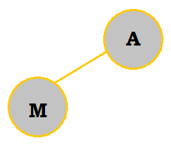
	AMERICAN starts with an A; thus, it is natural to make the tree's root an A.
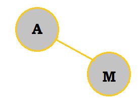	M is placed to the right of A because it comes later in the alphabet.
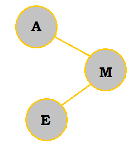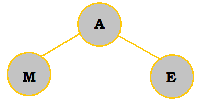
	E belongs on the right of A; however, because it comes before M in the alphabet, it is placed to the left of M.
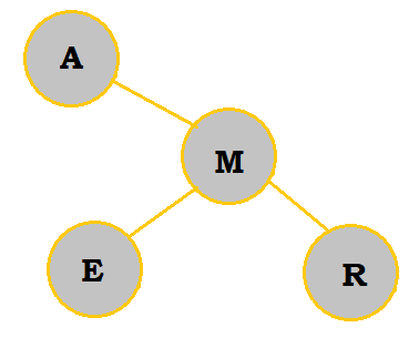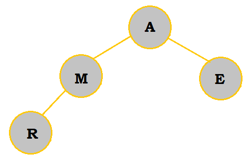
	R belongs on the right of A. Since it also comes after M, it is placed to the right of M.
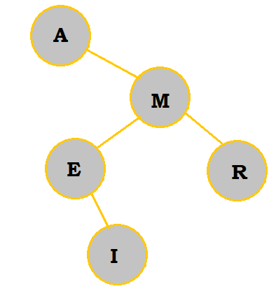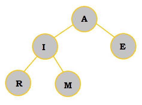
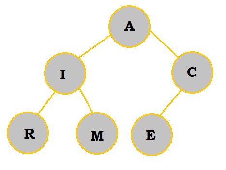
	I belongs on the right of A. It belongs to the left of M as well. I comes later in the alphabet than E, so I is placed to the right of E.
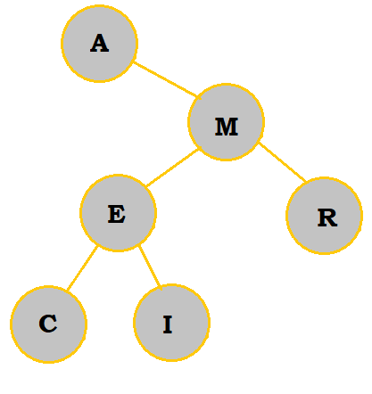	C belongs on the right of A and to the left of M. Since C comes before E, it is placed to the left.
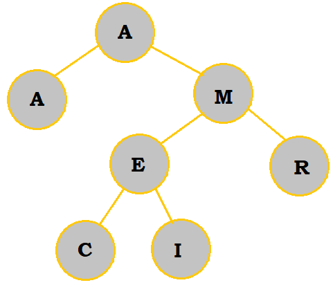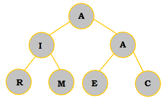
	A (the second one) is equal to the root A. So, it is placed to the left of the root.
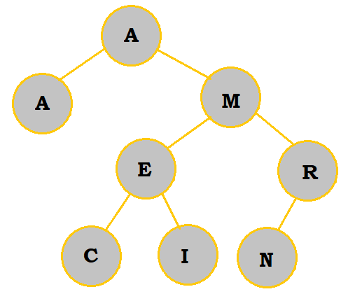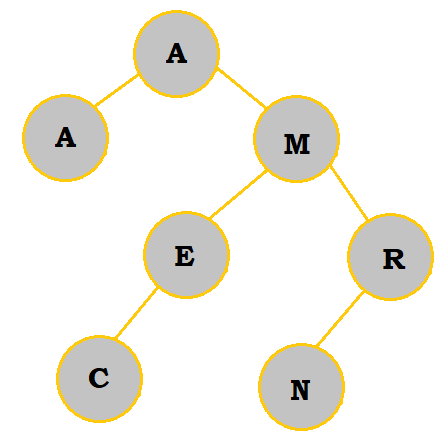
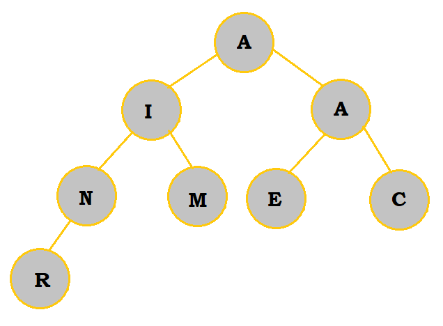
	N comes after A and M, so it belongs on the right of those. However, it is placed to the left of R, which comes even later.

Note that the order you insert the nodes does matter, so if you were to switch out the positions of the letters in AMERICAN to become something like MCEAANIR, the tree would look very different.

Deleting Nodes (Binary Search)

In the case that a node needs to be deleted, there are three cases you must consider: if the removed node has 0 children, 1 child, or 2 children. When there are no children, you can simply remove the node. When there is one child, move the child node and its children up to replace the parent node. When there are two children, move the left child and its children up to replace the parent node, and add on the right child and all of its children to the left child or its children, using the same comparison process as described above. Removing nodes generally involves some minor shifting because "less than or equal to" and "greater than" relationships between nodes still have to be considered for proper placement.

# of Children	Original	Deletion	Description
$0$			I has been removed. Since it had no children, no shifts needed to be made.
$1$			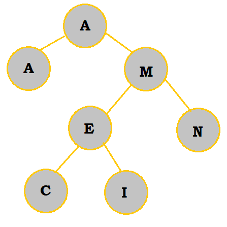R has been removed. Since it had 1 child, that child was moved up to be on the right of M. Since N comes after M, this shift is valid.
$2$			M has been removed. So, the left branch of M is moved up to take M's place. M's right branch is placed to the right of that branch.

Searching for Nodes

To search for a specific code, refer to the following pseudocode algorithm:

p = root
found = FALSE
while (p ≠ NIL) and (not found)
  if (x < p’s key)
    p = p’s left child
  else if (x > p’s key)
    p = p’s right child
  else
    found = TRUE
  end if
end while

So, searching first starts at the root of the tree and works its way down, moving either left or right based on what character you are searching for and where it is positioned within the tree. As an example, I will once again use the AMERICAN tree and attempt to find E.

First, p is set to the root, A. x holds the value we are trying to find, E.

Then, we move on to the while loop, whose conditions have both been met. In this loop, since E > p's key, p is then set to equal M. The cycle then ends, and we start the loop anew. This time, E < p's key, so p is now set to equal E. Note that the while loop does not stop here! Instead, it would traverse through the loop once again and then execute the "else" statement to make found = TRUE.

This algorithm should remind you of a binary search: check the parts of tree the greater than the current node if the node you are looking for is greater than the current node, or check the parts of the tree less than or equal to the current node if not.

So, by following this pseudocode, we have now successfully found our desired node.

Tree Traversal

Often times, storing inputs (namely in USACO Silver problems) for programming problems in a tree data structure is very advantageous. The following are two algorithms to traverse the tree data structure to search for a given node.

• Depth-First-Search
  • This technique is typically done with recursion and goes through each branch individually.
• Breadth-First-Search
  • This technique is done with a queue and adds the leaves of a branch to the end of the queue after each branch is done.

Classifying Trees Further

We've worked with the AMERICAN binary search tree for quite a while, and now let's analyze it a bit more just for good measure.

Balanced Trees

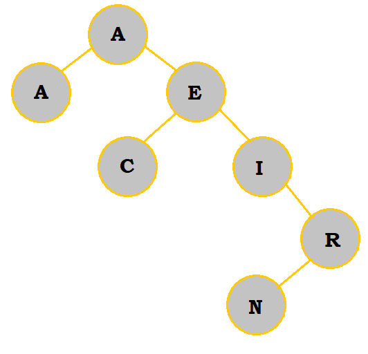
If we were to compare the left and right branches of the root, we can see that the left branch has significantly less nodes to work with, thus making the tree very unbalanced. The more unbalanced a tree is, the longer it takes to search for a node.

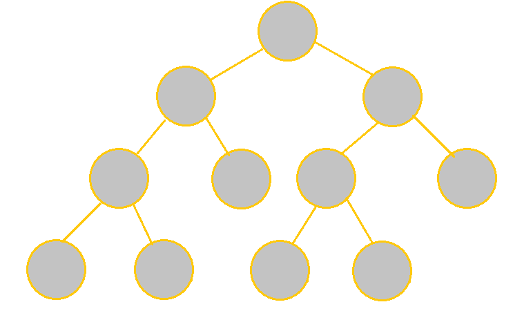
Let's compare these two images:

Unbalanced	Balanced

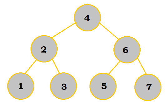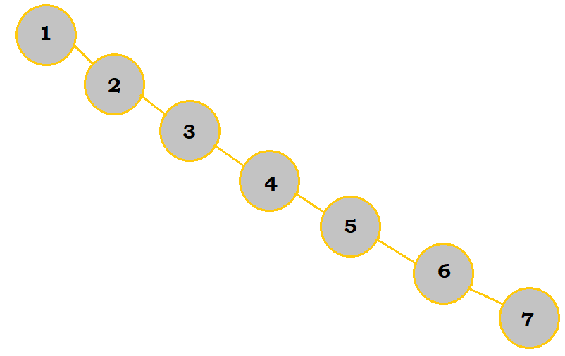
While these two trees display the same elements, they are drastically different because of the order the elements were put into the tree. If we wanted to search for 7 and used the pseudocode mentioned earlier in "Searching for Nodes", it would take us 7 loop cycles using the unbalanced tree to find it. On the other hand, it would only take us 3 cycles with the balanced tree because there were less "layers" to the tree to work with; that is why balanced trees are much more efficient overall.

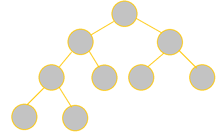
There is some leeway given to balanced trees; as long as the left and right branches of any particular node differ in the number of layers by no more than 1, then the tree is still considered balanced. See the image below:

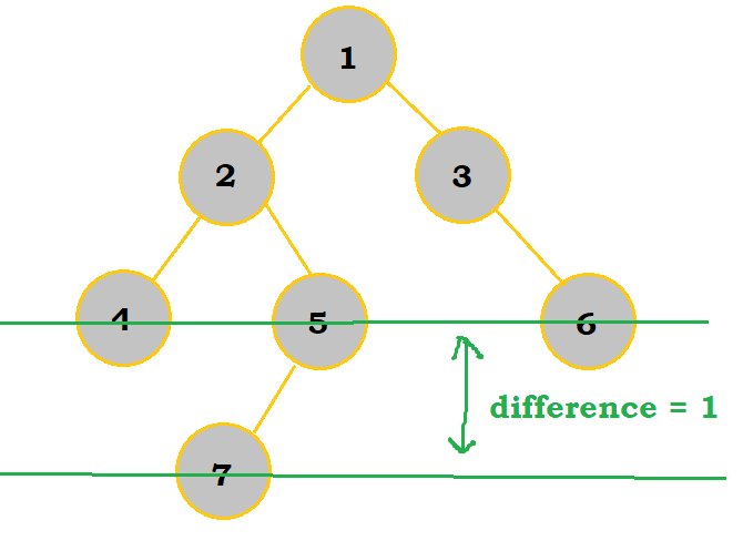
Although the tree leans more to the left subbranch, which has 4 elements compared to 2 in the right subbranch, this is still considered balanced as they only differ in 1 node layer overall.

Full vs Complete Trees

A Full tree, or strictly binary tree, is drawn in a way such that each node (except the leaves) has 2 nodes; they are not necessarily balanced. For complete trees, each level besides the last level must be filled. For the last level, while it does not need to be completely filled, any nodes in that level are all located on the left side.

See the table below to understand the differences between the two in more detail:

Tree	Description
	It is not complete because the last level's nodes are not all left-oriented. It is not full either because there is 1 node with only 1 child.
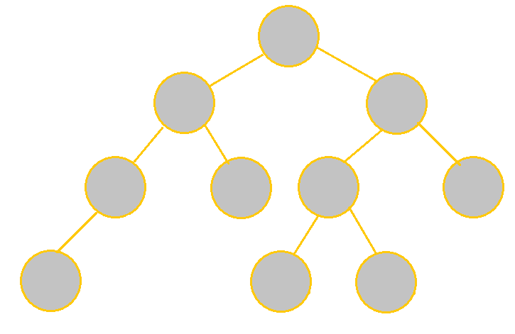
	It is complete because every level other than the last level is filled; the node in the last level is also oriented on the left. It is not full, however, because nodes cannot have only 1 child.
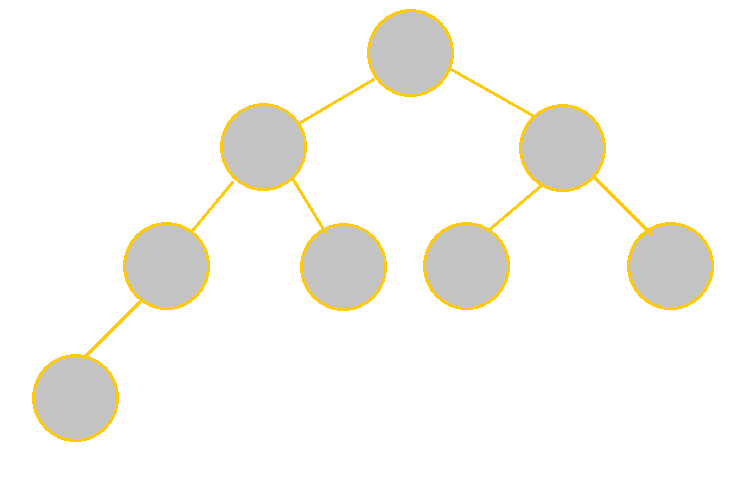
	It is full because each node indeed has 2 children besides the leaves. It is not complete because the nodes on the last level are not fully left-oriented.
	Each node has 2 children except for the leaves, so it is full. Each level is filled except for the last level, whose nodes are left-justified, thus making the tree complete.

Path Lengths

Before moving further into priority queues, let's talk briefly about path lengths. In earlier sections, we addressed "layers"/"levels" of the tree; these can also be referred to as "depths". The root node has a depth of 0; the next layer has a depth of 1, and this continues to increment for subsequent, deeper layers.

Internal path length (IPL) is the sum of the depths of all nodes in the tree. External path length (EPL) is the sum of the depths of the nodes that can be added to the tree's current leaves. An easier way to calculate the EPL is with this formula: EPL = IPL + 2n, where n represents the number of nodes in the tree.

IPL	EPL
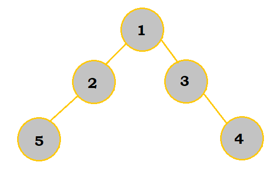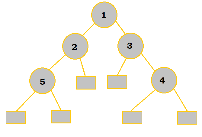
There are 5 nodes here. Node 1 has a depth of 0 since it's the root. Nodes 2 and 3 have a depth of 1 each. Nodes 4 and 5 have a depth of 2 each. So, the IPL = 0 + 2(1) + 2(2) = 6.	The squares represent the nodes that can be added to the tree. Two are of depth 2 while the other four are of depth 3. So, the EPL = 2(2) + 4(3) = 16. We could also solve this with the formula. Since the IPL is 6, and there are 5 nodes, the EPL = 6 + 2(5) = 16.

Priority Queues

Priority queues are similar to binary search trees. Essentially, elements that have the highest priority are served first, even if they may have been put into the queue much later. So, unlike binary search trees, inserting nodes may involve shifting other nodes to establish the priority order that we want.

With deleting and finding items, they are limited to the first item/element. While they are more limited, that does not mean they are necessarily worse than binary search trees; in some situations, deleting and finding other items may not be very important and thus can be ignored.

Inserting Nodes

Priority queues are typically implemented using a heap data structure. When using a min-heap, the parent is always less than or equal to its children nodes; the root is the smallest element in the tree. Conversely, a max-heap is where the parent is greater than or equal to its children nodes, and the root is the largest element in the tree.

As you add nodes, the tree is filled in from left to right, top to bottom; a level must be completely filled before moving onto the next one. Essentially, your heap must resemble a complete tree. When you add the node, you need to compare it with its parent. For min-heaps, if the new node is less than the parent, then you should switch the two and continue moving up the heap until the formation is valid. A similar idea applies to max-heaps except that it's for when the new node is greater than the parent. By doing so, all of the smallest elements (or largest for max-heap) would be at the top of the tree.

Take this table as an example on how to implement AMERICAN with a min-heap:

Step	Description
	A is added like normal as the root of the new tree.
	M is added as a child of A on the left end. Since M is larger than A, it stays where it is.
	E is added into the tree. No shifting of nodes occurs since E is indeed larger than A.
	R is added into the tree and starts the next row since the previous row was completely filled. No shifts occur because R is greater than M.
	I is first added as an child of M. However, because it is less than M, the two switch places. I is not less than A, so it does not move further up the heap.
	C is added as a child of E. However, since it is less than E, the two switch places. C is greater than A, so it does not switch places with the root.
	A (not the root) is added as a child of C. Since it is less than C, the two switch places. Since A has the same value as the root A, switching the two wouldn't be very useful, so the two As can be kept as is.
	N is added as a child of R and starts the next row. Since it is less than R, the two switch places. N is greater than I, it does not move further up the heap. We have now finished constructing the tree.

Deleting Nodes

Just as a reminder, only the root can be deleted! To do so, replace the root with the rightmost node in the last node layer. Then, keep switching out the root with its smaller child (or larger child, if using max-heap) until the tree is finally valid. Make sure to make adjustions to the rest of the tree if needed.

In the case that both of the root's children are smaller than the root itself, then choose the smallest child to replace the root with; of course, for max-heap, it would be that if both children are larger than the root, then the larger child should replace the root.

Sample Problems

1. Stacks/Queues: Determine what the value of C would be if the operations below were performed on an initially empty stack. Analyze it as a queue afterward.

PUSH(18)
B = POP()
PUSH(7)
PUSH(33)
C = POP()
A = POP()

As a stack… 18 would first be added to the stack; this would then be popped out and stored in B. Afterwards, 7 and 33 (in that order) are put into the stack. Because 33 was pushed into the stack later than 7, it is also the first to be popped; so, 33 is popped and stored into C, whereas 7 is stored in A. So, our final answer is 33.

As a queue… 18 would be added first; then, this would be popped out and stored in B. Afterwards, 7 and 33 (in that order) are put into the queue. Since queues follow a "first in, first out" rule, 7 would be popped first and stored into C. 33 would consequently be stored in A. So, our final answer here would be 7.

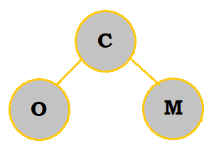
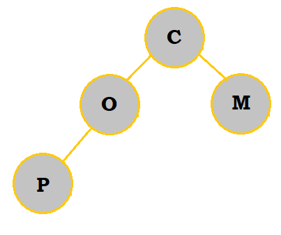
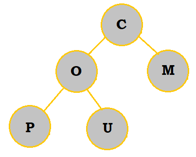
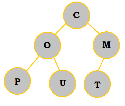
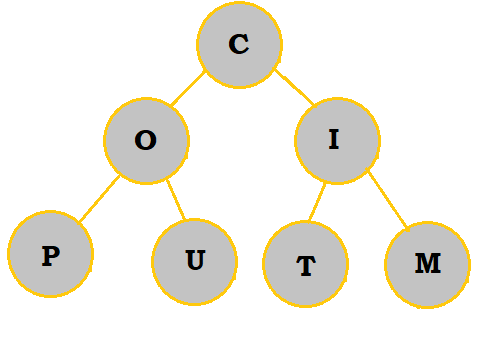
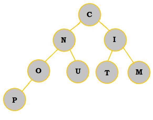
2. Create a priority queue of the letters COMPUTING with a min-heap. What are the letters in the bottommost row, from left to right?

Follow the table below to see how the priority queue is constructed:

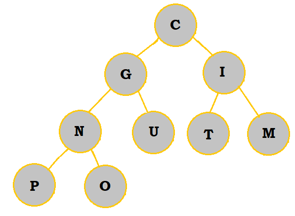So, the bottommost letters are P and O.

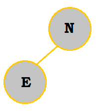
3. Create a binary search tree with the letters NEUQUA. What are the internal path length and external path length?

Follow the table below to see how the binary search tree is constructed:

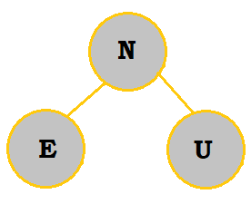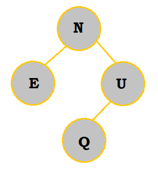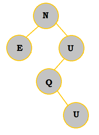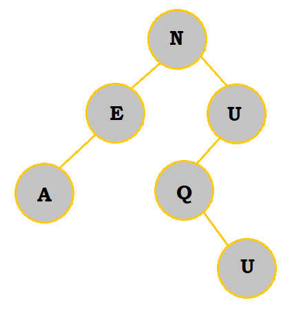The internal path length would be 0 + 2(1) + 2(2) + 3 = 9. The external path length would be 9 + 2(6) = 21.

---

Authors: Kelly Hong, Raymond Zhao